USF Information Science Blog

Question 1:

Question 2:

Question 3:

Question 4:

A. Consider a population consisting of the following values, which represents the number of ice cream purchases during the academic year for each of the five housemates.

8, 14, 16, 10, 11

a. Compute the mean of this population.

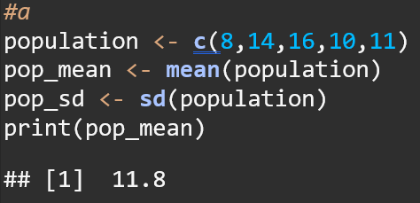
The mean of this population is 11.8

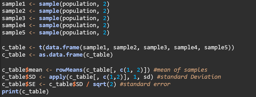
b. Select a random sample of size 2 out of the five members. See the example used in the Power-point presentation slide # 13.

The randomly selected values of the 5 ended up being 8 and 11

c. Compute the mean and standard deviation of your sample.

The mean of the sample population is 9.5. The standard deviation of the sample population is 2.12132

d. Compare the Mean and Standard deviation of your sample to the entire population of this set (8,14, 16, 10, 11).

B. 

Suppose that the sample size n = 100 and the population proportion p = 0.95.

1. Does the sample proportion p have approximately a normal distribution? Explain.

To determine if a sample size will have approximately normal distribution, the following needs to be calculated based on the Central Limit Theorem: The sample size n should be large enough so that both n*p and n*(1−p) both greater than or equal to 5 (Note: Some versions of the CLT recommend these values to be higher, such as 10 or even 15 in some cases, these are more conservative estimates, and I’ve found the general rule of thumb to be 5, so I will be using 5 as the threshold for these calculations).

n*p = 100*0.95 = 95
n*(1−p) = 100*(1-0.95) = 5

Since both of these conditions are met, the sample proportion has approximately normal distribution according to the central limit theorem.

2. What is the smallest value of n for which the sampling distribution of p is approximately normal?   

According to the central limit theorem, both n*p and n*(1−p) needs to be greater than 5, so both equations need to be solved for n, and the highest value taken.

n*0.95=5
n = 5/0.95 = 5.26

n*(1−0.95) = 5
n*(0.05) = 5
n = 5/0.05 = 100

The smallest value where both conditions are satisfied is n = 100, as 100 is the smallest value of n that can be used when p = 0.95

The sample mean  from a group of observations is an estimate of the population mean u. Given a sample of size n, consider n independent random variables X1, X2, …, Xn, each corresponding to one randomly selected observation. Each of these variables has the distribution of the population, with mean u and standard deviation σ .

A. Population mean= (8­­+14+16+10+11) / 5 = 11.8

B. Sample of size n = 5 because the population has five different values 

C. Mean of sample distribution, standard deviation, and Standard Error

D. I am looking for table with the following variables X, x=u, and (x-u)^2

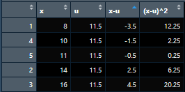
C. Simulated coin tossing: is probability better done using function called rbinom() than using function called sample()?  Explain.

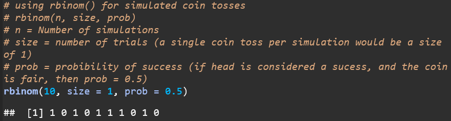
Advantages of rbinom():

• rbinom is specifically designed for probabilistic experiments. It is built to handle binary outcomes, making it ideal for tasks like simulating coin tosses or similar experiments.
• Generates outcomes according to the binomial distribution. The function automatically applies the probability distribution without needing extra setup.
• Effective for large simulations. rbinom() efficiently handles simulations with many trials, making it well-suited for larger datasets.

Limitations of sample():

• Not specialized for probabilistic experiments. While it can be used for simulations, sample() is a more general-purpose function and lacks the specialized focus of rbinom().
• Requires more manual setup. You need to define probabilities and conditions explicitly, which can make sample() more cumbersome compared to rbinom() for probability-based simulations.

Question 1:

A. State the null and alternative hypothesis
Null Hypothesis (H₀):
The mean breaking strength of cookies produced by the new machine is equal to the specified mean of 70 pounds.
H₀ ​: μ = 70

Alternative Hypothesis (H₁):
The mean breaking strength of cookies produced by the new machine is different from the specified mean of 70 pounds.
H₁ : μ ≠ 70

B. Is there evidence that the machine is not meeting the manufacturer’s specifications for average strength? Use a 0.05 level of significance

This code shows that the null hypothesis cannot be rejected because the calculated z-score falls within the range of the critical z-values, indicating that there is not enough evidence to suggest that the machine’s mean cookie strength significantly differs from the manufacturer’s specified mean.

C. Compute the p value and interpret its meaning

The p-value is approximately 0.0719. The p-value represents the probability of obtaining a test statistic at least as extreme as the one observed (in this case, a z-score of approximately -1.80), assuming the null hypothesis is true. Since the p-value (0.0719) is greater than the significance level (α=0.05), we do not have enough evidence to reject the null hypothesis. If the p-value was less than 0.05 (the significance level), it would indicate that the observed data is statistically significant, meaning the likelihood of obtaining the observed result, assuming the null hypothesis is true, is very low.

D . What would be your answer in (B) if the standard deviation were specified as 1.75 pounds?

This code shows that the null hypothesis should be rejected because the calculated z-score falls outside the range of the critical z-values, indicating that there is evidence to suggest that the machine’s mean cookie strength significantly differs from the manufacturer’s specified mean.

E. What would be your answer in (B) if the sample mean were 69 pounds and the standard deviation is 3.5 pounds?

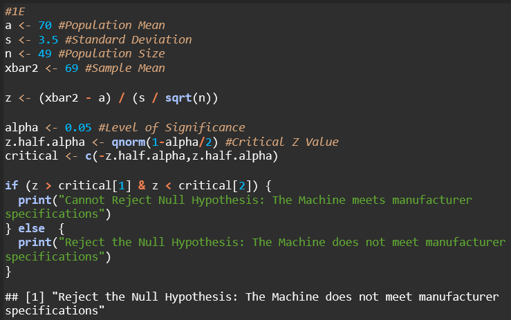
This code shows that the null hypothesis should be rejected because the calculated z-score falls outside the range of the critical z-values, indicating that there is evidence to suggest that the machine’s mean cookie strength significantly differs from the manufacturer’s specified mean.

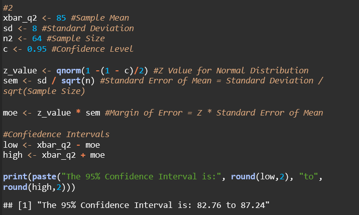
Question 2:
If x̅ = 85, σ = standard deviation = 8, and n=64, set up 95% confidence interval estimate of the population mean μ.

Question 3:
Data Manipulation and Munging:

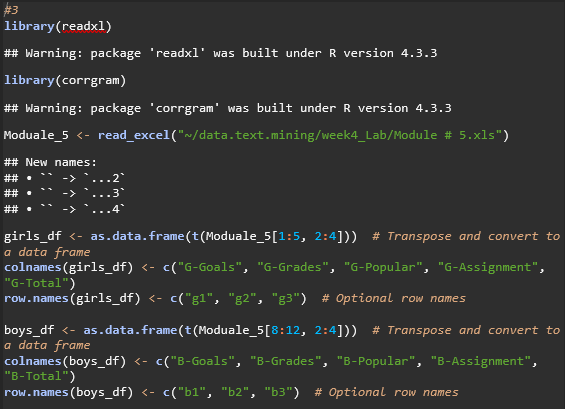
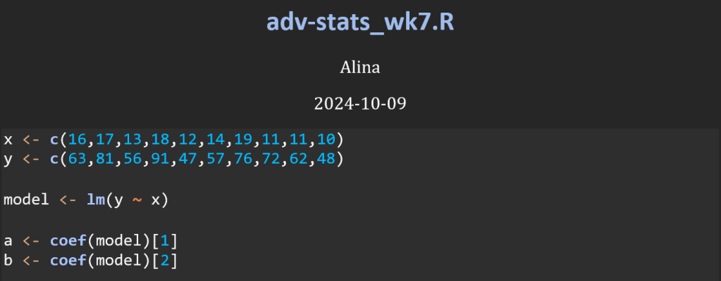
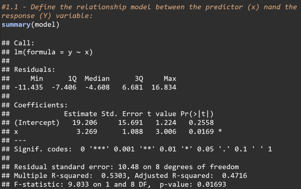
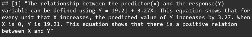
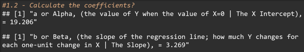
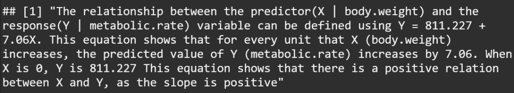
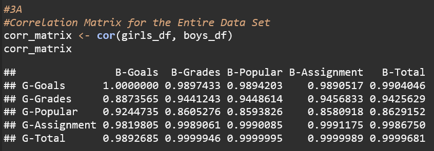
A.  Calculate the correlation coefficient for this data set

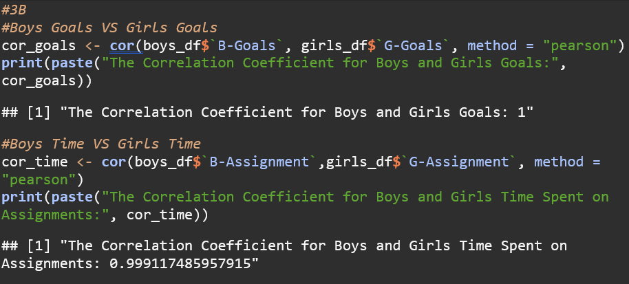
B.  Pearson correlation coefficient for x= girls and y =boys. (goals, time spend on assignment)

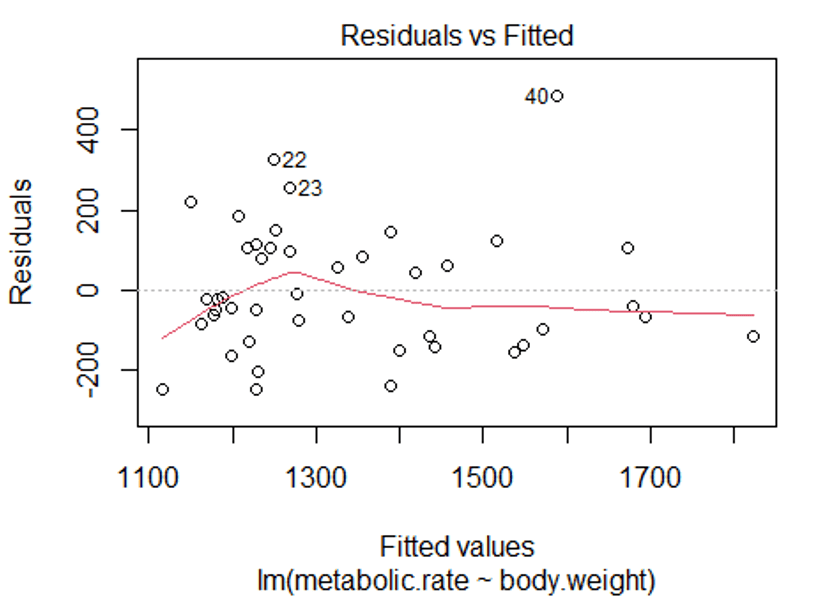
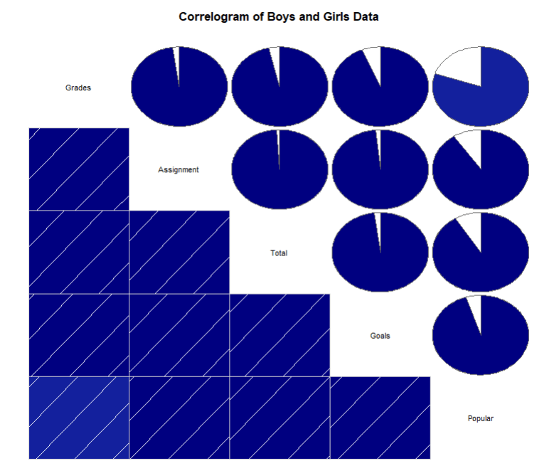
C.  Create plot of the correlation

A1. Event A
The probability of Event A is (10+20)/90 = 0.3333 (1/3)

A2. Event B?
The probability of Event B is (10+20)/90 = 0.3333 (1/3)

A3. Event A or B
To find the probability of A or B, we use the formula:
P(A∪B)=P(A)+P(B)−P(A∩B)

P(A∩B) is equal to the probability of Event A and B
The probability of Event A and B is 10/90 = 0.1111 (1/9)

The probability of Event A OR B is (1/3)+(1/3)-(1/9)=0.5556 (5/9)

A4. P(A∪B)  = P(A) + P(B)
The formula P(A∪B)  = P(A) + P(B) only holds true when events A and B are mutually exclusive, meaning they cannot happen at the same time. For this chart, A and B are not mutually exclusive, as they can occur concurrently.

However, if events A and B are not mutually exclusive, the formula becomes: P(A∪B)=P(A)+P(B)−P(A∩B) (which was used in A3)

When events A and B are not mutually exclusive, they may both occur at the same time. Therefore, the intersection P(A∩B) (the probability that both A and B happen together) is subtracted to avoid double-counting.

B. Applying Bayes’ Theorem 

B1. Is this answer True or False.
This conclusion is true

B2. Please explain why?

P( A1 ) = 5/365 =0.0136985 [It rains 5 days out of the year.]
P( A2 ) = 360/365 = 0.9863014 [It does not rain 360 days out of the year.]
P( B | A1 ) = 0.9 [When it rains, the weatherman predicts rain 90% of the time.]
P( B | A2 ) = 0.1 [When it does not rain, the weatherman predicts rain 10% of the time.]

We are trying to find the probability of there being rain on Janes weddings given the weatherman predicts rain: P(A1​∣B). Bayes Theorem can be written as such:

N: P(A1​)⋅P(B∣A1​)​
D: P(A1​)⋅P(B∣A1​)+P(A2​)⋅P(B∣A2​)

N: P(A1​)⋅P(B∣A1​) = 0.0136985×0.9 = 0.0123287
D: P(A1​)⋅P(B∣A1​)+P(A2​)⋅P(B∣A2​) = 0.0123287+0.09863014 = 0.11095879

P(A1​∣B) = 0.11095879 / 0.01232865​ = 0.1111 , or, 11.11%

The probability that it rains on any given day in the desert is very low: only 5/365≈1.37%. This means that, despite the accuracy of the weatherman’s prediction rate, the base rate of rain is still quite low. Since it rarely rains, most of the days when the weatherman predicts rain, it actually won’t rain. This is why the final probability is much lower than the weatherman’s accuracy for predicting rain. In conclusion, the result is True because the calculation is based on accurate probabilities and follows Bayes’ Theorem correctly, but the seemingly low probability reflects the rarity of rain in the desert, despite the weatherman’s forecast.

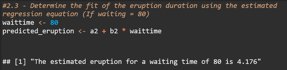
C. Last assignment from our textbook, pp. 55 Exercise # 2.3.

This is a binomial probability problem, where:

• size=10 (the number of patients),
• prob=0.80 (the probability of no complications for each patient),
• x=10 (the number of patients with no complications).

[1] 0.1073742

The probability of of operating on 10 patients successfully with the tradtional method is 10.73%

The following are two sets of data – each consist of 7 observations (n=7).

Set#1:  10, 2, 3, 2, 4, 2, 5

Set#2:  20, 12, 13, 12, 14, 12, 15

1. For each set, compute the mean, medium, and mode under Central Tendency

2. For each set, compute the range, interquartile, variance, standard deviation under Variation

3. Compare your results between set#1 vs. set #2 by discussing the differences between the two sets.

4. Post your result and discussion on your blog.

When I first began this assignment, I started with consulting the R reference card for functions in R so I could find each of the functions I needed to complete this assignment. I was able to find all the functions I needed on the ref card except for a function to calculate the Most Frequent, or mode, of the values. After conducting some further research, I discovered that R does not have a built in function to calculate mode, so I began this assignment with inputting set 1 and 2 into R, as well as writing a custom function to find the mode of the sets.

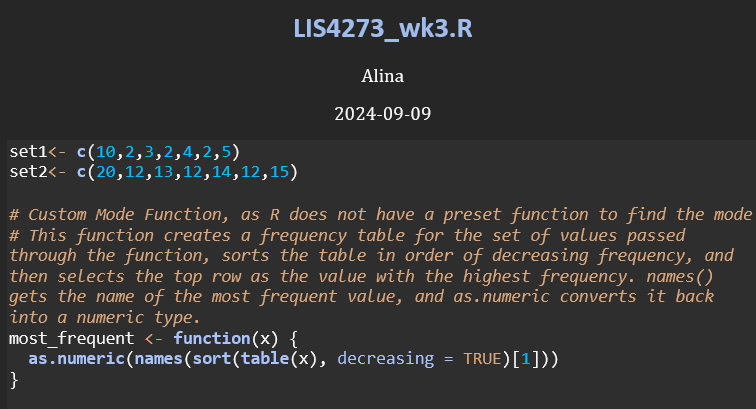
I called this function most_frequent(), as R already has a function called mode(); however, R’s mode() function does not return the most frequent value, but rather it returns the storage mode or the data type of an object, such as “numeric”, “character”, “logical”, etc.. When I tried using mode() during this assignment, it returned “numeric”. While helpful when developing my custom function for finding the most frequent value in the datasets, this was not what I was trying to find for this assignment.

With both sets of data input into R and my custom function for finding the most frequent value written, I was able to begin the assignment.

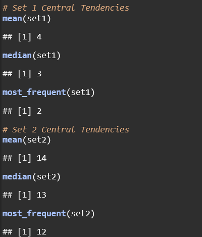
1. Compute the Mean, Median, and Mode for both data sets

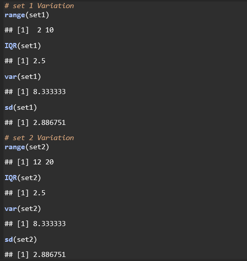
2. Compute the range, interquartile, variance, standard deviation for both data sets

3. Compare your results between set#1 vs. set #2

Something I noticed when I was inputting the values for set 1 and 2 was that the values of set 2 were simply the values of set 1 + 10. Because I noticed this, I was not surprised when the Mean, Median, and Mode of Set 2 was exactly 10 units higher than Set 1 across all central tendencies (Mean: 4 vs. 14, Median: 3 vs. 13, Mode: 2 vs. 12). However, what I was surprised about was that the measure of variation did not change at all from set 1 to set 2.

Both sets have the same range (8 units), the interquartile range (IQR) was 2.5 for both sets, as well as identical variance (8.333) and standard deviation (2.887). These identical data variations confirm that the shift by 10 did not affect the spread of the data, and that the spread of data points relative to their respective means remained unchanged.

What this tells me is that uniform shifts in data sets (such as, adding 10 to all values, for example), impacts central measures of tendency, but not variability. Both sets share identical statistical properties regarding spread (range, variance, standard deviation), emphasizing that adding a constant affects position but not dispersion.

4. Post your result and discussion on your blog

Completed September 9th, 2024

1. I have downloaded the outline instructions for how to import data into RStudio. I think this is a great reference for how to important multiple data types and formats into R and look forward to having it on hand for future assignments

2. I was actually very surprised when I first looked at our Introductory Statistics with R textbook, as I had just completed a certificate on Datacamp that referenced and discussed the precedents set by this publication. Much of what was discussed in Chapter 1 was familiar to me, as I took Introduction to Data Science in the Spring 2024, but it was a welcome refresher after a summer away from RStudio, especially the section on difference data and object types.

However, in regard to The Art of R programming, one thing I was surprised to learn was that R is considered object-oriented programing. Suddenly, my mental comparisons between R and Java make a lot more sense, and I realize why USF wanted me to take an object-oriented programing course before i jumped into my data science core.

Of the two textbooks, I enjoyed reviewing The Art of R programming the most.

3. Your assignment, evaluate the following function call myMean. The data for this function called assignment. The assignment contains the following data:  6, 18, 14, 22, 27, 17, 19, 22, 20, 22.

The first line of this code creates a vector called assignment2, which holds the values 6, 18, 14, 22, 27, 17, 19, 22, 20, 22. The second line of code creates a function called myMean, which takes the argument ‘assignment2’, and then returns the mean (The Sum divided by the Length) of the values. The final line of the code runs the function myMean, using the vector assignment2 as the argument. The mean of assignment2 is reported to be 18.7

myMean is a custom function created by the user to calculate the mean of a group of values. It efficiently computes the average by summing all values in the vector and dividing by the count of values.

 What is the meaning behind the term’s statistics? And analytics?

According to the dictionary, Statistics are pieces of numerical data. Statistics, as the discipline, refers to collecting proportions of data and using that collected data to make mathematically supported inferences about the whole. Analytics refers to the systematic computational processes of making those mathematically supported inferences.

What is R programming language?
The R programming language is the programming language used in RStudio. It is specifically used for statistical computation and data visualization. R is an open-source and free programming language that has been adopted by many industries outside of Statistics.