USF Information Science Blog

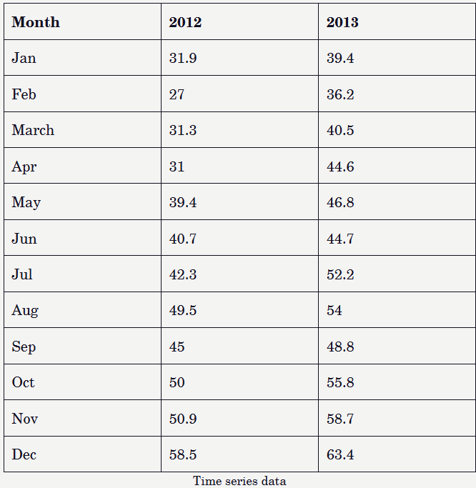
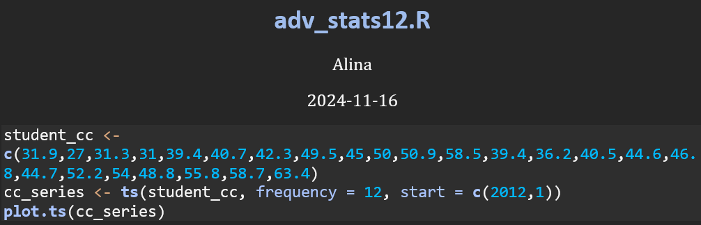
This code imports the data, transforms it into a time-series object, and generates a plot to visualize the changes in values over a 24-month period, spanning from January 2012 to December 2013.

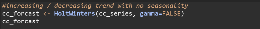
This chart shows a general upward trend throughout the year, followed by a drop at the start of the next. However, due to the limited duration of the dataset, this does not necessarily indicate seasonality. Seasonality refers to recurring patterns observed consistently over multiple cycles, such as daily, monthly, or yearly intervals. Because we can only see two cycles in this data, we cannot assume seasonality. Since we are assuming that the data lacks clear seasonality, we will use Holt-Winter’s exponential smoothing technique with the seasonality parameter (gamma) set to False.

Smoothing parameters:
Alpha = This is the smoothing parameter for the level. A high alpha (closer to 1) indicates that the model gives more weight to recent observations when updating the level.
Beta = A lower beta value suggests that the trend is smoothed more slowly compared to the level, making it less sensitive to fluctuations in the trend over time.
Gamma = Indicates that seasonal smoothing is turned off, meaning the model does not include a seasonal component.

Coefficients
a: This represents the smoothed estimate of the level (the overall “baseline” value of the time series).
b: This represents the smoothed estimate of the trend (the rate of change over time). It indicates that, on average, the values are increasing by approximately 2.43 units per time period.

This chart demonstrates the results of Holt-Winters exponential smoothing, with the black line representing the observed (actual) values of the time series, and the red line representing the fitted (smoothed) values from the model.

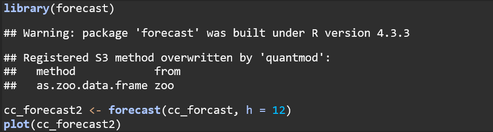
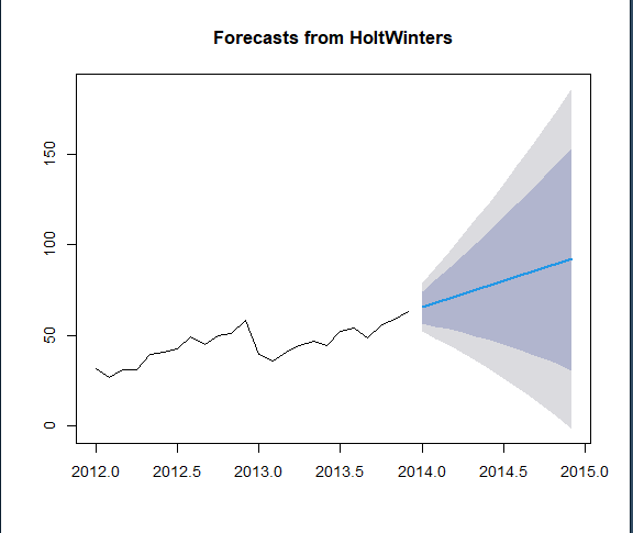
This plot displays the results of forecasting using the Holt-Winters model for the next 12 time periods. The black line represents the historical observed data, while the blue line and shaded areas represent the forecast and confidence intervals, with 80% prediction intervals shown in the dark blue section, and 95% prediction intervals shown in the light grey.

Discussion on Time Series Models
The results of the Exponential Smoothing Model using Holt-Winters effectively captured the upward trend in the time series data while smoothing out short-term fluctuations. The fitted values closely aligned with the observed data, providing a clear representation of the underlying trend. The sharp dip in 2013 is assumed to be an anomaly, as we lack sufficient data to determine if it reflects a recurring seasonal trend. While it is possible that a similar dip could occur at the beginning of 2014, there is currently no evidence to support this pattern. Thus, we proceed under the assumption that this dip is an anomaly until additional intervals provide further clarification.

Time series analysis is invaluable for tracking changes in variables over fixed intervals across a duration of time. The Holt-Winters smoothing technique and the forecast library in R can help predict future values by emphasizing recent observations, incorporating trends, and accounting for potential seasonality. Forecasting models offer significant advantages over standard linear or polynomial regression when working with time series data. One key strength of forecasting models is their ability to capture temporal dynamics, recognizing that recent observations often have a stronger influence on future values than older data. Standard regression, by contrast, assumes independence between observations, which is often unrealistic in time series contexts.