USF Information Science Blog

The code essentially sets up an additive model to analyze the effect of the treatment (treat), the period of administration (period), and individual differences between subjects (subject) on the VAS scores. The attach() function allows us to reference ashina column names without specifying ashina$ each time. This additive model is designed to capture the effects of the treatment, period, and subject (individual differences) on the VAS score.

(Intercept): This is the baseline level (subject 1) when treat and period are set to their baseline levels. The estimate of -113.06 suggests a VAS score starting point (when all factors are at baseline) and is significantly different from zero (Pr(>|t|) < 0.001).
Subject Coefficients (subject2, subject3, etc.): These represent the difference in VAS score for each subject relative to the baseline subject (subject1). For instance:

• subject2 has a coefficient of 51.50, indicating that their VAS score is expected to be 51.50 higher than the baseline (subject1) after controlling for other factors. However, this estimate is not statistically significant (Pr(>|t|) = 0.190721).
• Significant values have stars (e.g., subject3, subject4, etc.), indicating that these subjects’ VAS scores are significantly different from the baseline.

Treat: The treatment effect shows that moving from the placebo (coded as 0) to the active treatment (coded as 1) decreases the VAS score by -42.87. This effect is statistically significant (Pr(>|t|) = 0.005491), meaning the active treatment is likely effective in reducing the VAS score compared to placebo.
Period: This coefficient has NA for its estimate, standard error, t-value, and p-value. This suggests singularity, which occurs when there is perfect multicollinearity—meaning one or more predictor variables can be exactly predicted from others in the model. Here, period is likely collinear with other factors (like subject or treat), so it cannot be estimated separately. This often happens in repeated measures data where the model is over-specified.

Model Summary:
Residual standard error: This is the average distance that the observed VAS scores fall from the model’s predicted scores.
Multiple R-squared (0.7566): This indicates that approximately 75.66% of the variance in VAS scores is explained by the model.
Adjusted R-squared (0.4969): This adjusts for the number of predictors in the model. Here, it’s quite a bit lower, indicating that some predictors may not be adding substantial explanatory power.
F-statistic and p-value: The F-test evaluates the overall significance of the model. A p-value of 0.02229 indicates that, overall, the model fits the data better than a model with no predictors.

T-value: This is the calculated t-statistic, which measures the difference between the means relative to the variability in the data. A larger absolute t-value indicates a larger difference between the two groups.
P-value: A p-value of 0.005644 suggests that this difference is statistically significant at the 0.05 level (and even at the 0.01 level), meaning we reject the null hypothesis that there is no difference between the two treatments.
Confidence Interval: This confidence interval shows the range within which the true mean difference is likely to fall 95% of the time. Since both bounds of the interval are negative, this further indicates that the active treatment is associated with a reduction in VAS scores compared to the placebo.
Mean Difference: The mean difference between vas.active and vas.plac is -42.875. This aligns with the treatment effect in the linear model output, where the coefficient for treat was also around -42.87, indicating consistency between the two analyses.

Comparison between the t.tests and lm() models:
The paired t-test provides a direct comparison between the active and placebo treatments, while the additive model (from lm) also considers individual subject differences and the period of treatment. Both methods show a similar treatment effect, but the additive model gives additional insights by accounting for these extra factors.

These matrices show how each term (main effects and interaction) is represented in the design matrix for the respective model. The difference between ~ a * b and ~ a : b lies in which terms are included in the model:

~ a * b

• This shorthand expands to ~ a + b + a:b.
• It includes:
  • Main effects for both a and b (individual contributions of a and b to the response variable).
  • Interaction effect a:b (the combined effect of specific levels of a and b).
• This formulation is useful when you want to assess both the independent effects of each factor and how they interact with each other.

~ a : b

• This includes only the interaction term a:b.
• It does not include main effects for a or b individually.
• This model assumes that the effect of a and b on the response variable exists only through their interaction. It does not model the individual effects of a and b separately.

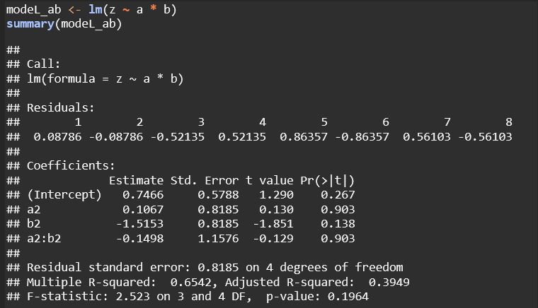
Model z ~ a * b: This is a more comprehensive model, including both main effects and interaction terms. It avoids singularities and allows for independent interpretation of each factor and their combined effects. Although none of the terms are statistically significant here, the model structure is more flexible and interpretable.

Model z ~ a : b: This model only includes the interaction between a and b without main effects, which led to a singularity (NA for a2:b2). It’s less robust and restricts interpretation, making it harder to assess the individual contributions of a and b.