USF Information Science Blog

A. Consider a population consisting of the following values, which represents the number of ice cream purchases during the academic year for each of the five housemates.

8, 14, 16, 10, 11

a. Compute the mean of this population.

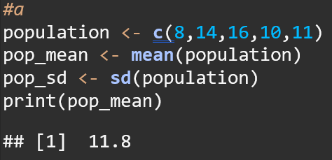
The mean of this population is 11.8

b. Select a random sample of size 2 out of the five members. See the example used in the Power-point presentation slide # 13.

The randomly selected values of the 5 ended up being 8 and 11

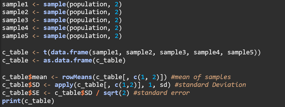
c. Compute the mean and standard deviation of your sample.

The mean of the sample population is 9.5. The standard deviation of the sample population is 2.12132

d. Compare the Mean and Standard deviation of your sample to the entire population of this set (8,14, 16, 10, 11).

B. 

Suppose that the sample size n = 100 and the population proportion p = 0.95.

1. Does the sample proportion p have approximately a normal distribution? Explain.

To determine if a sample size will have approximately normal distribution, the following needs to be calculated based on the Central Limit Theorem: The sample size n should be large enough so that both n*p and n*(1−p) both greater than or equal to 5 (Note: Some versions of the CLT recommend these values to be higher, such as 10 or even 15 in some cases, these are more conservative estimates, and I’ve found the general rule of thumb to be 5, so I will be using 5 as the threshold for these calculations).

n*p = 100*0.95 = 95
n*(1−p) = 100*(1-0.95) = 5

Since both of these conditions are met, the sample proportion has approximately normal distribution according to the central limit theorem.

2. What is the smallest value of n for which the sampling distribution of p is approximately normal?   

According to the central limit theorem, both n*p and n*(1−p) needs to be greater than 5, so both equations need to be solved for n, and the highest value taken.

n*0.95=5
n = 5/0.95 = 5.26

n*(1−0.95) = 5
n*(0.05) = 5
n = 5/0.05 = 100

The smallest value where both conditions are satisfied is n = 100, as 100 is the smallest value of n that can be used when p = 0.95

The sample mean  from a group of observations is an estimate of the population mean u. Given a sample of size n, consider n independent random variables X1, X2, …, Xn, each corresponding to one randomly selected observation. Each of these variables has the distribution of the population, with mean u and standard deviation σ .

A. Population mean= (8­­+14+16+10+11) / 5 = 11.8

B. Sample of size n = 5 because the population has five different values 

C. Mean of sample distribution, standard deviation, and Standard Error

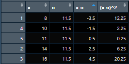
D. I am looking for table with the following variables X, x=u, and (x-u)^2

C. Simulated coin tossing: is probability better done using function called rbinom() than using function called sample()?  Explain.

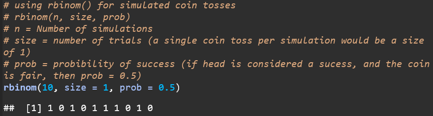
Advantages of rbinom():

• rbinom is specifically designed for probabilistic experiments. It is built to handle binary outcomes, making it ideal for tasks like simulating coin tosses or similar experiments.
• Generates outcomes according to the binomial distribution. The function automatically applies the probability distribution without needing extra setup.
• Effective for large simulations. rbinom() efficiently handles simulations with many trials, making it well-suited for larger datasets.

Limitations of sample():

• Not specialized for probabilistic experiments. While it can be used for simulations, sample() is a more general-purpose function and lacks the specialized focus of rbinom().
• Requires more manual setup. You need to define probabilities and conditions explicitly, which can make sample() more cumbersome compared to rbinom() for probability-based simulations.